High-Level Review (Previous Post)
Entire project (Please note: this flow chart is constantly being updated)
Current project (Please note: this flow chart is constantly being updated)
Sub-project (Please note: this flow chart is constantly being updated)
Current Project: Computational Design of Foldable Robotic Body
-
Here are some comparisons of FEA and the method I choose to use
(1) A pros and cons comparison of FEA and the method I choose to use
| FEA | Our Approach | |
|---|---|---|
| Pros | (1) Modeling of complex geometries and irregular shapes are easier as varieties of finite elements are available for discretization of domain. (2) Boundary conditions can be easily incorporated in FEM. (3) Different types of material properties can be easily accommodated in modeling from element to element or even within an element. (4) Higher order elements may be implemented. (5) FEM is simple, compact and result-oriented and hence widely popular among engineering community. |
(1) Suitable for calculating modeling of complex geometries and irregular shapes, but with faster speed. (2) Boundary conditions are even easier to apply than FEA. (3) Material properties (Young's modulus, Possion's ratio, thickness) are easy to incorporate. (4) Faster calculation due to the relatively small amount of linear calculations needed. (5) Accessible to non-expert users due to the ease of use. (6) A lot less computational power needed to operate. (7) Easy to provide loading conditions. |
| Cons | (1) Large amount of data is required as input for the mesh used in terms of nodal connectivity and other parameters depending on the problem. (2) It requires a digital computer and fairly extensive. (3) It requires longer execution time. |
(1) Lower accuracy compared with FEA. (2) Currently limited to isotropic materials with uniform thickness. (3) Only uniform stress results across thickness direction. |
(2) An approach comparison of FEA and the method I choose to use
| FEA | Our Approach | |
|---|---|---|
| Method | (1) Discretization or subdivision of the domain. (2) Selection of the interpolation functions (to provide an approximation of the unknown solution within an element). (3) Formulation of the system of equations. (4) Solution of the system of equations |
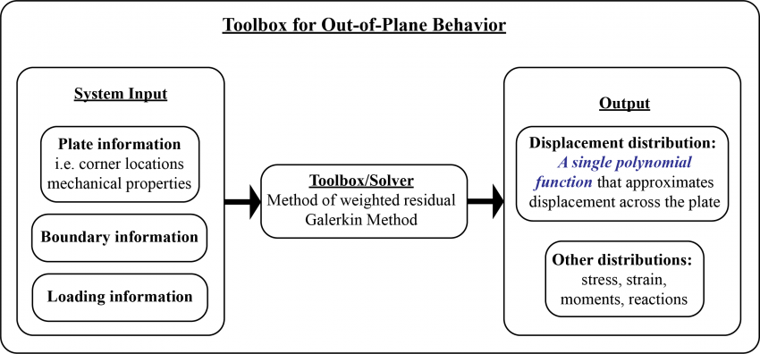
(1) Define displacement functions (across the entire plate) as polynomial functions, e.g. \(\omega_{(x, y)} = \sum_{i=1}^{k} c_i \varphi_{i(x,y)}\) and \(\varphi_{i(x,y)}\) are polynomial functions. (2) Using different techniques to solve the 4th order plate bending governing equations, e.g. method of weight residual and minimum of potential energy method. (3) Solve polynomial coefficients, \(n\) linear equations. (4) Calculate other results, such as stress, strain, moments and reaction load, by simply applying corresponding partial differential equations. |
| Computational complexity / calculation time | Displacement of each nodes need to be solved independently. Depending on the amount of node selected, computation can be very complex. | Only need to solve a limited amount of coefficients, resulting in a limited amount of linear equations to be solved, which is relatively fast to compute using even a 'regular computer'. |
Current Project Breakdowns
Entire project
Out-of-plane analysis //Done//
-
(1) System high-level flow chart
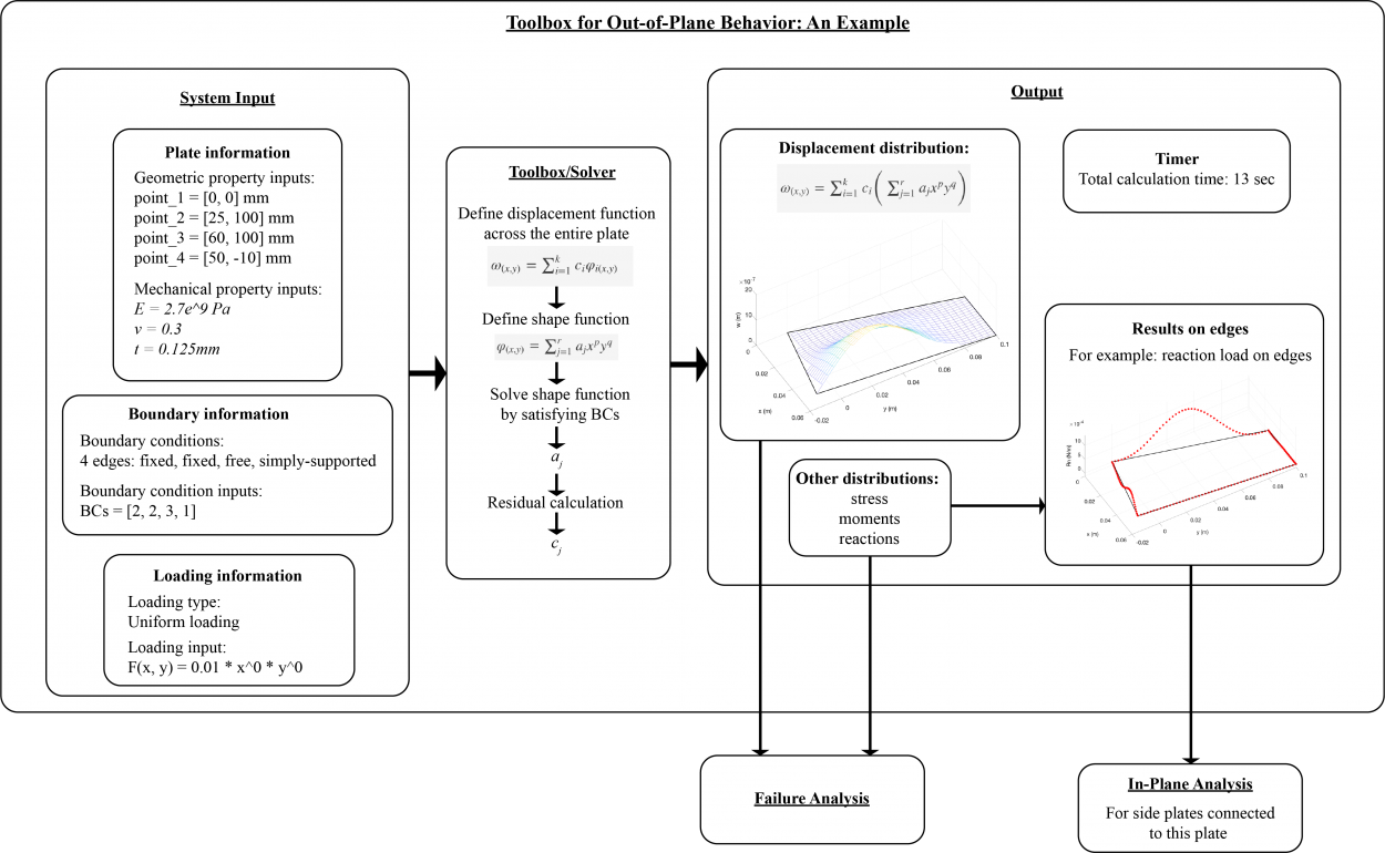
(2) An example case
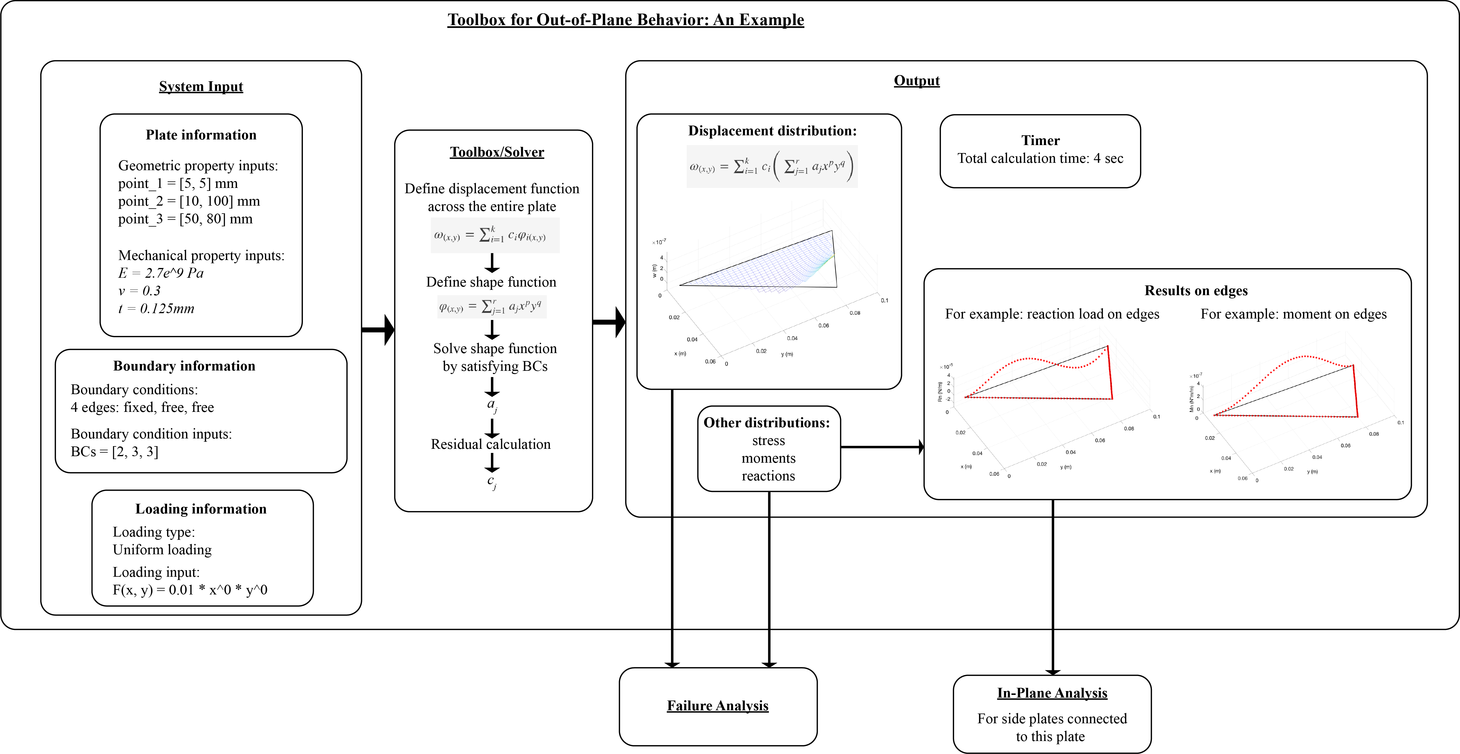
(3) A second example case: triangle with only one edge fixed
(4) Plans for this part of the project.
We can wrap it up, find a good demonstration/application (possibly with furniture/chair design), and submit to a conference paper.
In-plane analysis //On-going//
The in-plane analysis for those side plates follows the same logics as the analysis of out-of-plane behavior:
-
Plate deformation will be approximate as one function of (x, y) over the entire plate.
-
Instead of using method of weighted residual, method of minimum potential energy is applied.
-
Results are polynomial equations, approximating deformations. Other variables, e.g. stress distribution, can be calculated using the deformation polynomial equation.
Plans for the near future
-
Write a research proposal for the up-coming year.
-
Figure out a potential application/demonstration for what I have done now and summarize it into a paper and submit. I will talk to Wenzhong and June to see if we can applies what I have done to furniture design.
-
Help Wenzhong finish his IROS.
-
Discuss with Pehuen for potential projects.
Detailed Method Write-ups
(1) Plate Analysis of Out-of-Plane Loading (Previous Post)
The method used here to study the out-of-plane bending is call method of weight residual (MWR).
Method Write-up
The thin plate governing differential equation for the deflections:
\(\frac{\partial^4 \omega_{(x, y)}}{\partial x^4} + 2 \frac{\partial^4 \omega_{(x, y)}}{\partial x^2 \partial y^2} + \frac{\partial^4 \omega_{(x, y)}}{\partial y^4} = \frac{P_{(x, y)}}{D}\)
\(\frac{\partial^4 \omega_{(x, y)}}{\partial x^4} + 2 \frac{\partial^4 \omega_{(x, y)}}{\partial x^2 \partial y^2} + \frac{\partial^4 \omega_{(x, y)}}{\partial y^4} = \nabla^{4}\omega_{(x, y)}\)
Base function (deflection function in this case):
\(\omega_{(x, y)} = \sum_{i=1}^{k} c_i \varphi_{i(x,y)}\)
Using \(n^{th}\) 2D polynomial transformations to build shape (trial) function \(\varphi_{(x,y)}\):
\(\varphi_{(x,y)} = \sum_{j=1}^{r} a_j x^{p} y^{q}\)
\(p + q \leq n\)
\(r = \frac{(n+1)(n+2)}{2}\)
Parameters \(a_j\) can be solved by applying boundary conditions to shape (trial) function \(\varphi_{(x,y)}\).
Residual function:
\(R_{(x,y)} = \nabla^{4}\omega_{(x, y)} - \frac{P_{(x, y)}}{D}\)
\(R_{(x,y)} = \sum_{i=1}^{k} c_{i} \nabla^{4} \varphi_{(x, y)} - \frac{P_{(x, y)}}{D}\)
Using Galerkin method to calculate coefficient \(c_i\):
\(\big( R_{(x,y)}, \varphi_{(x, y)} \big) = 0\)
\(\int\int R_{(x,y)} \varphi_{(x, y)} dx dy = 0\)
Once we have all parameters (\(a_j\), \(c_i\)) solved, we will get an approximate solution to the plate governing differential equation:
\(\omega_{(x, y)} = \sum_{i=1}^{k} c_i \bigg( \sum_{j=1}^{r} a_j x^{p} y^{q} \bigg)\)
Once a deflection function \(\omega_{(x,y)}\) has been determined, the stress resultants in terms of deflections can be calculated as follows
\(M_x = -D \bigg( \frac{\partial^2 \omega}{\partial x^2} + \nu \frac{\partial^2 \omega}{\partial y^2} \bigg)\)
\(M_y = -D \bigg( \frac{\partial^2 \omega}{\partial y^2} + \nu \frac{\partial^2 \omega}{\partial x^2} \bigg)\)
\(M_{xy} = -D (1 - \nu) \frac{\partial^2 \omega}{\partial x \partial y}\)
The vertical forces (shear forces) are
\(V_x = - D \frac{\partial}{\partial x} \bigg( \frac{\partial^2 \omega}{\partial x^2} + \frac{\partial^2 \omega}{\partial y^2} \bigg)\)
\(V_y = - D \frac{\partial}{\partial y} \bigg( \frac{\partial^2 \omega}{\partial x^2} + \frac{\partial^2 \omega}{\partial y^2} \bigg)\)
The reactive loads are
\(R_x = V_x - \frac{\partial M_{xy}}{\partial y}\)
\(R_y = V_y - \frac{\partial M_{xy}}{\partial x}\)
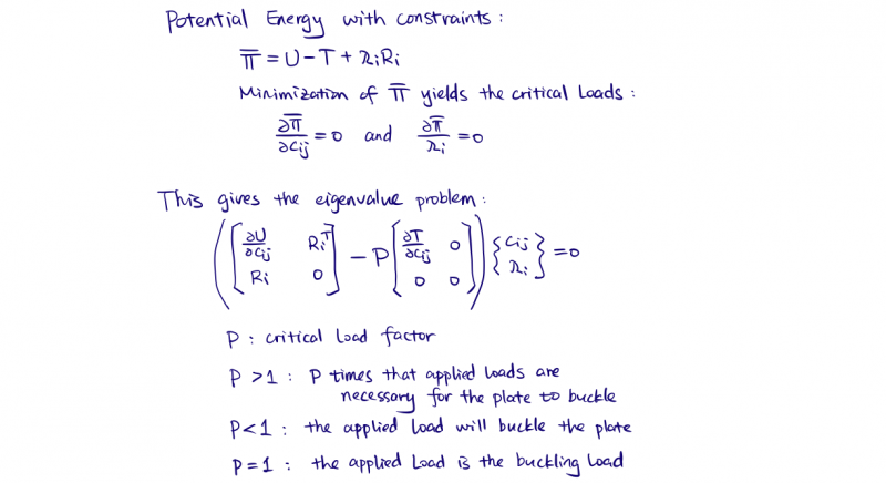
(2) Plate Analysis of In-Plane Loading (Previous Post)
The method used here to study the buckling is call minimum potential energy method.
Step 1: Subparametric Mapping in FEA System. (I have no background in this, so it took a while to get the information I needed and some time to learn this knowledge.)
-
Goal: This is for transforming irregular shaped plane into square shape in another coordinate system. This will make integration easier.
-
See details in my note here.
-
I studied 'subparametric mapping'. From Cartesian domian into (\(\zeta\), \(\eta\)) domain.
-
A figure of (\(\zeta\), \(\eta\)) domain, a quadrilateral element:

-
For a polygon, with number of edges no greater than 8, we can use 8-node mapping method to change coordinates from Cartesian domian into (\(\zeta\), \(\eta\)) domain. I did not get the same result as that presented in the paper. I assume it is because the node sequence I use is different than the one used in the paper, which is not clearly stated. But my result also make sense. I will use the result from this paper in my later calculation.
-
The reason for doing this mapping is for easy integration in later steps.
-
A good reference can be found here if you want to learn. Here is another one about quadrilateral element. Here is a useful website.
Step 2: Plane Stress, Strain Energy U Calculation.
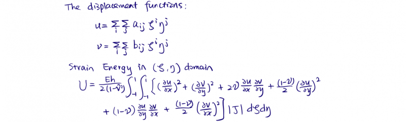
- See details in my note here.
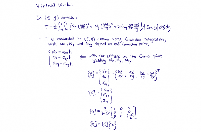
Step 3: Plane Stress, Virtual Work Energy T Calculation.

- See details in my note here.
Step 4: Solving Coefficients Using Minimum Potential Energy Method.
- Goal: get in-plane displacement \(u\) and \(v\), in order to get plane stress and strain. This plane stress and strain will be later applied to calculate bucalking virtual work energy. The reason to do it this way is because, for irregular shaped polygon, it is hard to calculate loading conditions on edges.
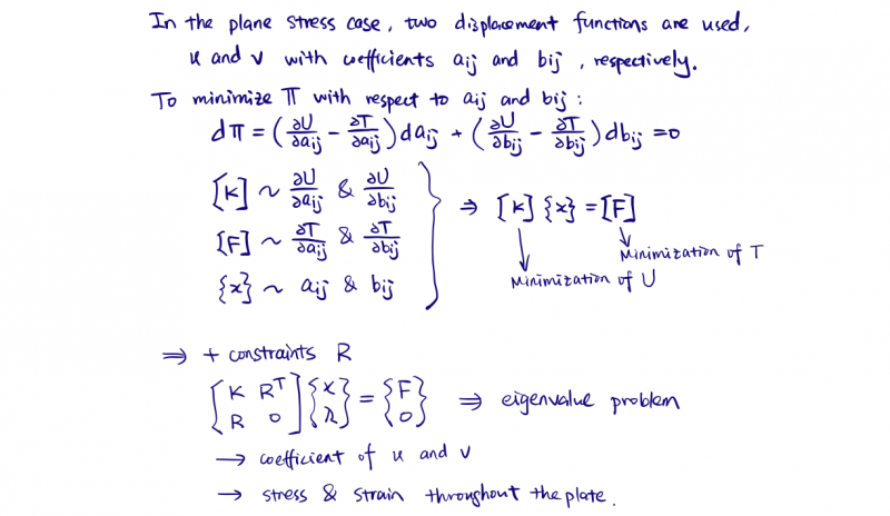
- Detailed calculation steps / validations on Lagrange multiplier are shown below:
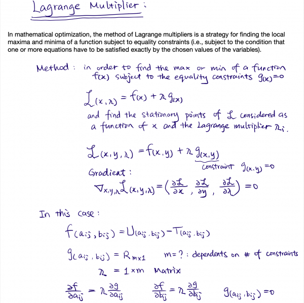
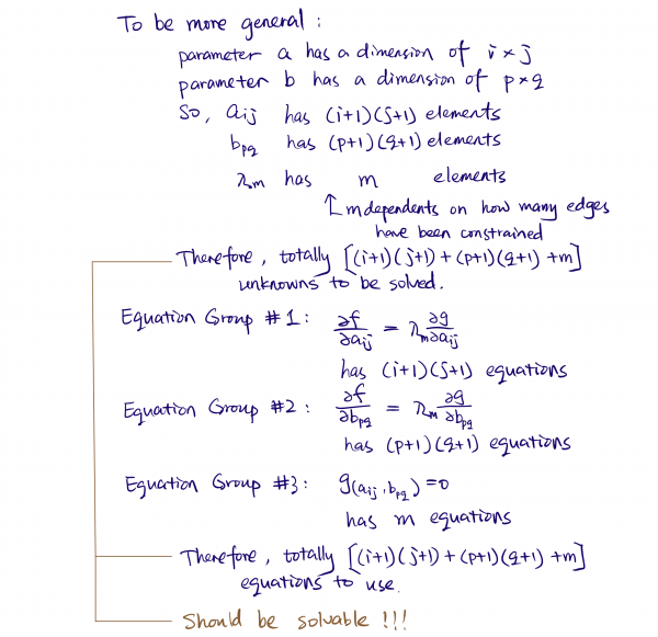
- See details in my note here.
Step 5: Buckling (Bending), Strain Energy U Calculation.

-
A full derivative of \(\frac{\partial \zeta}{\partial x}\), \(\frac{\partial \zeta}{\partial y}\), \(\frac{\partial \eta}{\partial x}\) and \(\frac{\partial \eta}{\partial y}\) can be solved using a method called implicit derivative and using Mathemetica, results can be found here.
-
See details in my note here.
Step 6: Buckling (Bending), Virtual Work Energy T Calculation.
- See details in my note here.
Step 7: Solving Coefficients Using Minimum Potential Energy Method.
- Goal: calculate buckling load (coefficients).
- See details in my note here.