Identifying weak points and failure modes in foldable structures, different methods exploration
Chang LiuMethod of Weighted Residuals + Galerkin Method
"Reduce the continuous-system mathematical model to a discrete idealization."
"In applied mathematics, methods of mean weighted residuals (MWR) are methods for solving differential equations. The solutions of these differential equations are assumed to be well approximated by a finite sum of test functions. In such cases, the selected method of weighted residuals is used to find the coefficient value of each corresponding test function. The resulting coefficients are made to minimize the error between the linear combination of test functions, and actual solution, in a chosen norm." [Ref]
Method Write-up
The thin plate governing differential equation for the deflections:
\(\frac{\partial^4 \omega_{(x, y)}}{\partial x^4} + 2 \frac{\partial^4 \omega_{(x, y)}}{\partial x^2 \partial y^2} + \frac{\partial^4 \omega_{(x, y)}}{\partial y^4} = \frac{P_{(x, y)}}{D}\)
\(\frac{\partial^4 \omega_{(x, y)}}{\partial x^4} + 2 \frac{\partial^4 \omega_{(x, y)}}{\partial x^2 \partial y^2} + \frac{\partial^4 \omega_{(x, y)}}{\partial y^4} = \nabla^{4}\omega_{(x, y)}\)
Base function (deflection function in this case):
\(\omega_{(x, y)} = \sum_{i=1}^{k} c_i \varphi_{i(x,y)}\)
Using \(n^{th}\) 2D polynomial transformations to build shape (trial) function \(\varphi_{(x,y)}\):
\(\varphi_{(x,y)} = \sum_{j=1}^{r} a_j x^{p} y^{q}\)
\(p + q \leq n\)
\(r = \frac{(n+1)(n+2)}{2}\)
Parameters \(a_j\) can be solved by applying boundary conditions to shape (trial) function \(\varphi_{(x,y)}\).
Residual function:
\(R_{(x,y)} = \nabla^{4}\omega_{(x, y)} - \frac{P_{(x, y)}}{D}\)
\(R_{(x,y)} = \sum_{i=1}^{k} c_{i} \nabla^{4} \varphi_{(x, y)} - \frac{P_{(x, y)}}{D}\)
Using Galerkin method to calculate coefficient \(c_i\):
\(\big( R_{(x,y)}, \varphi_{(x, y)} \big) = 0\)
\(\int\int R_{(x,y)} \varphi_{(x, y)} dx dy = 0\)
Once we have all parameters (\(a_j\), \(c_i\)) solved, we will get an approximate solution to the plate governing differential equation:
\(\omega_{(x, y)} = \sum_{i=1}^{k} c_i \bigg( \sum_{j=1}^{r} a_j x^{p} y^{q} \bigg)\)
Once a deflection function \(\omega_{(x,y)}\) has been determined, the stress resultants in terms of deflections can be calculated as follows
\(M_x = -D \bigg( \frac{\partial^2 \omega}{\partial x^2} + \nu \frac{\partial^2 \omega}{\partial y^2} \bigg)\)
\(M_y = -D \bigg( \frac{\partial^2 \omega}{\partial y^2} + \nu \frac{\partial^2 \omega}{\partial x^2} \bigg)\)
\(M_{xy} = -D (1 - \nu) \frac{\partial^2 \omega}{\partial x \partial y}\)
The vertical forces (shear forces) are
\(V_x = - D \frac{\partial}{\partial x} \bigg( \frac{\partial^2 \omega}{\partial x^2} + \frac{\partial^2 \omega}{\partial y^2} \bigg)\)
\(V_y = - D \frac{\partial}{\partial y} \bigg( \frac{\partial^2 \omega}{\partial x^2} + \frac{\partial^2 \omega}{\partial y^2} \bigg)\)
The reactive loads are
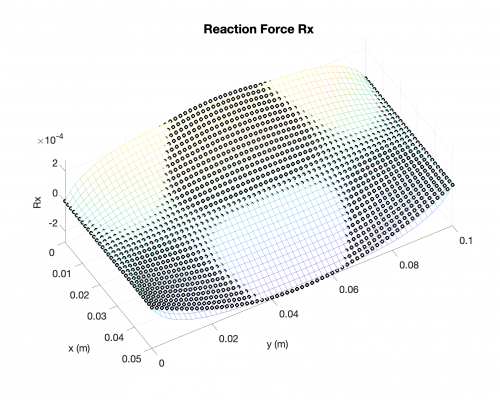
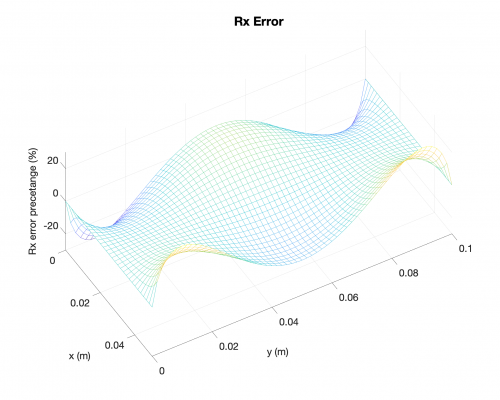
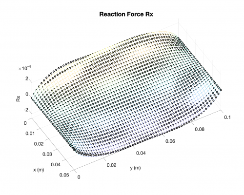
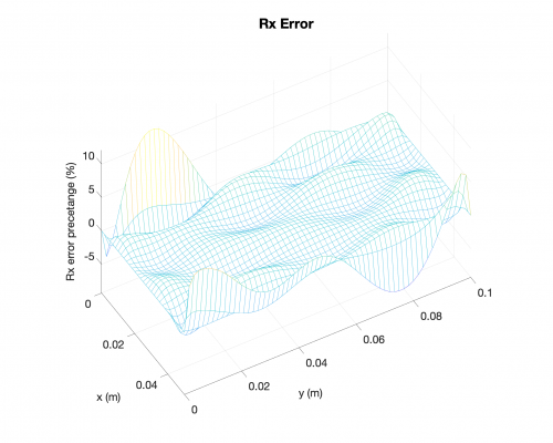
\(R_x = V_x - \frac{\partial M_{xy}}{\partial y}\)
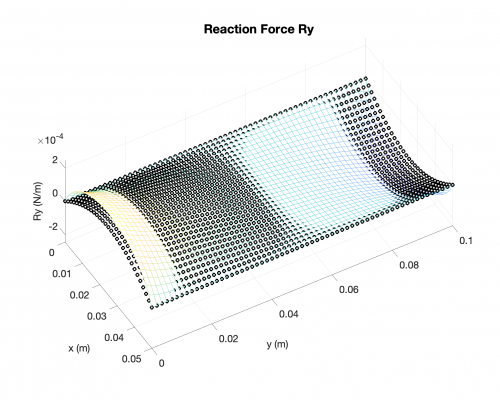
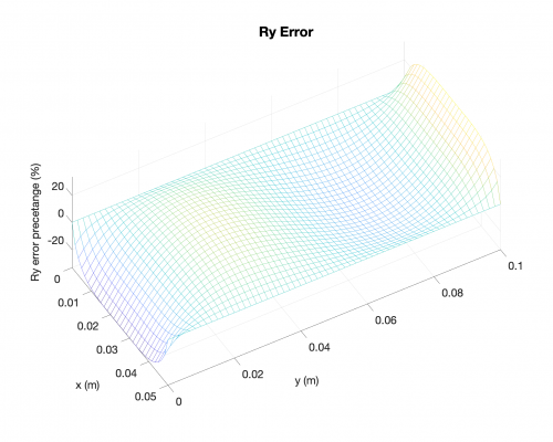
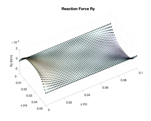
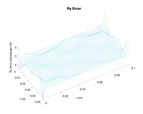
\(R_y = V_y - \frac{\partial M_{xy}}{\partial x}\)
Computational Implementation
In the following link, you will find an implementation for the following case:
-
Shape: rectangle
-
Boundary conditions: simply supported on all edges
-
Loading condition: distributed load across the plate
-
Comparison: yes, with existing analytical solution
See link here for rectangle+distributeload+SSSS
In the following link, you will find an implementation for the following case:
-
Shape: rectangle
-
Boundary conditions: clamped on all edges
-
Loading condition: distributed load across the plate
-
Comparison: no, unfortunately, there is no existing analytical solution
See link here for rectangle+distributeload+CCCC
- Special note: the reason why I keep using rectangle shape with distrubuted loading condition and simply supported boundary conditions is because it exists well-defined (and implemented) analytical (exact) solution. Other cases do not have this privilege. After we get FEA (presumably ABAQUS) up and runing, we can work on more generalized cases (arbitrary shapes, arbitrary boundary conditions and arbitrary loading conditions).
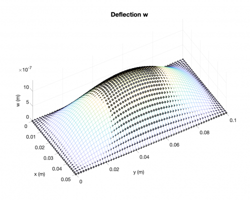
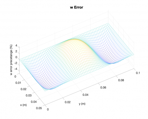
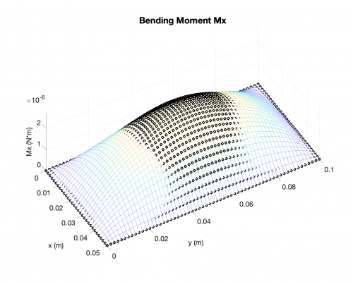
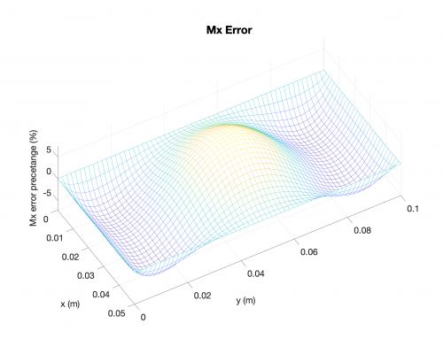
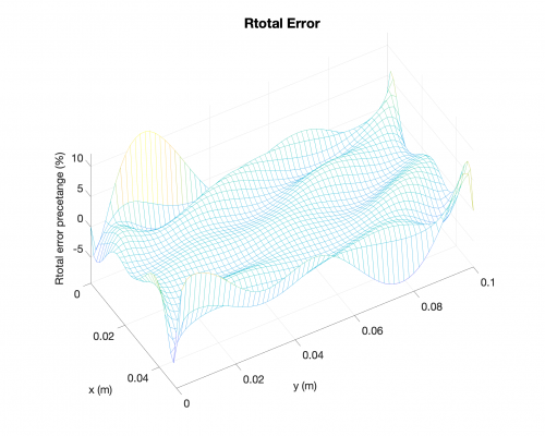
Example Results + Comparisons + Error Percetage
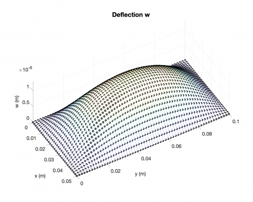
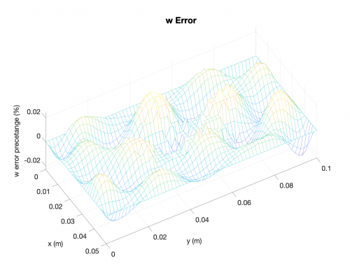
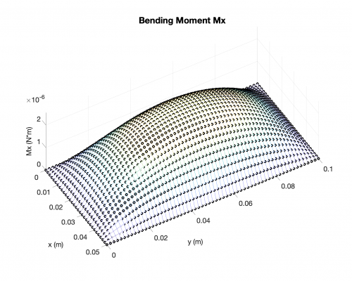
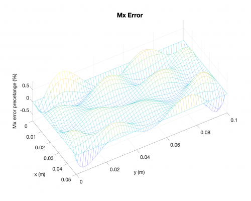
In the followings, you will find results for the following case:
-
Shape: rectangle
-
Boundary conditions: simply supported on all edges
-
Loading condition: distributed load across the plate
-
Polynomial order: 8 (minimum)
-
Calculation time: 3.6 sec
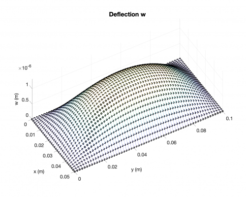
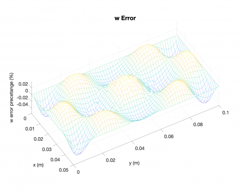
Deflection
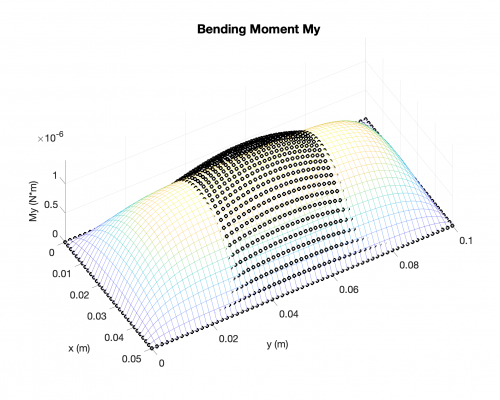
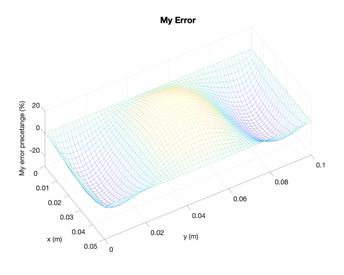
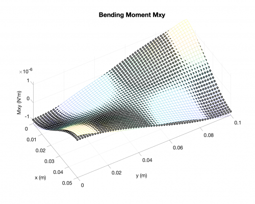
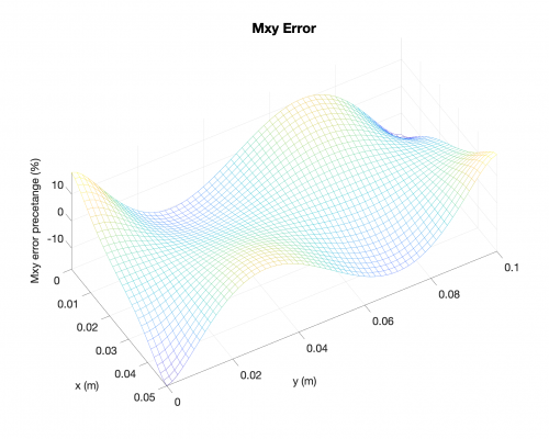
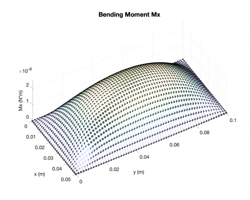
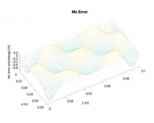
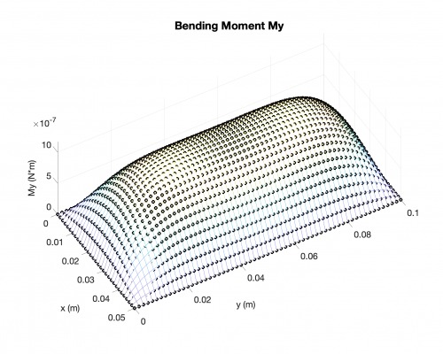
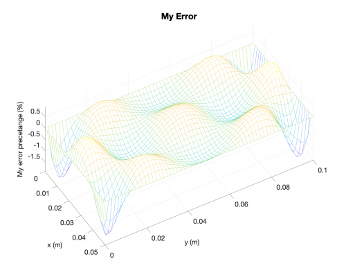
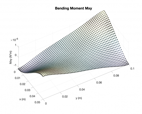
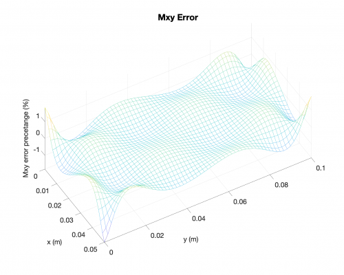
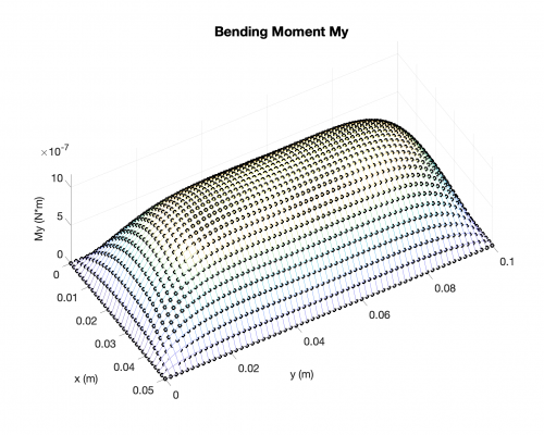
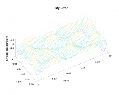
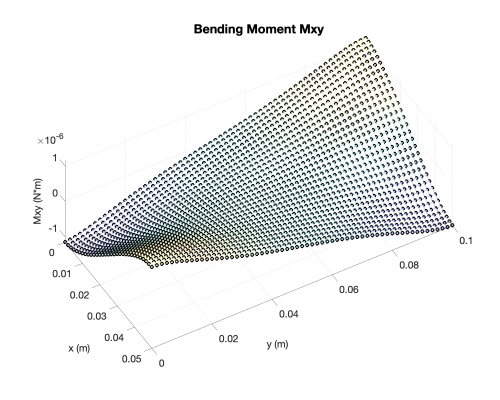
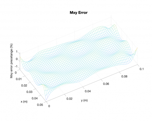
Bending Moments
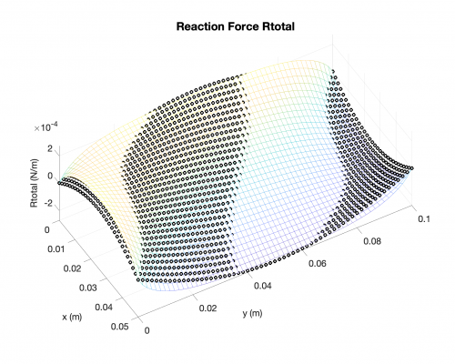
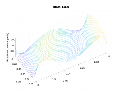
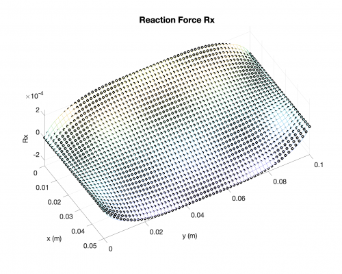
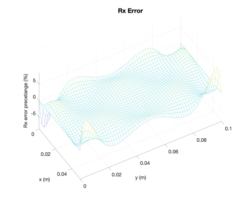
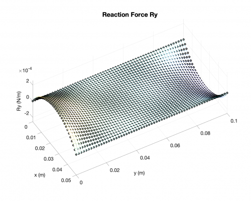
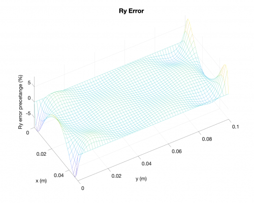
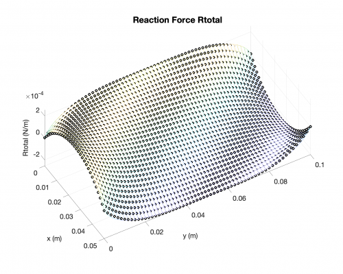
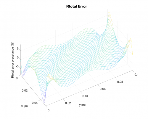
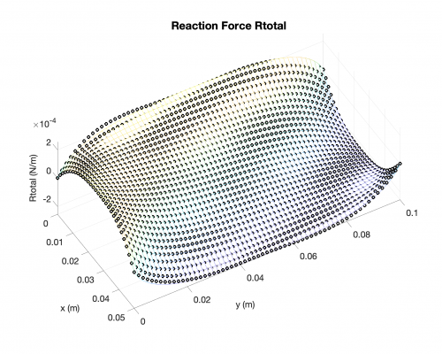
Reaction Forces
In the followings, you will find results for the following case:
-
Shape: rectangle
-
Boundary conditions: simply supported on all edges
-
Loading condition: distributed load across the plate
-
Polynomial order: 12
-
Calculation time: 25 sec
Deflection
Bending Moments
Reaction Forces
In the followings, you will find results for the following case:
-
Shape: rectangle
-
Boundary conditions: simply supported on all edges
-
Loading condition: distributed load across the plate
-
Polynomial order: 16
-
Calculation time: 255 sec
-
"Warning: Matrix is close to singular or badly scaled. Results may be inaccurate."
Deflection
Bending Moments
Reaction Forces
Questions
-
How to find the lowest possible polynomial (\(n\)) to satisfy the boundary conditions?
-
A higher order of polynomial will make better convergence. How much higher is enough for us? How does increasing order of polynomial influence the computational efficienty?
-
How many shape functions do we need / will we get?
-
How to implement boundary conditions when edges are not parallel to either coordinate?
-
How to determine 'computational complexity'?
Useful links:
Boundary Value Problems
Trial function / shape function
"Shape functions are selected to fit as exact as possible the Finite Element Solution. If this solution is a combination of polynomial functions of nth order, these functions should include a complete polynomial of equal order."