Goal
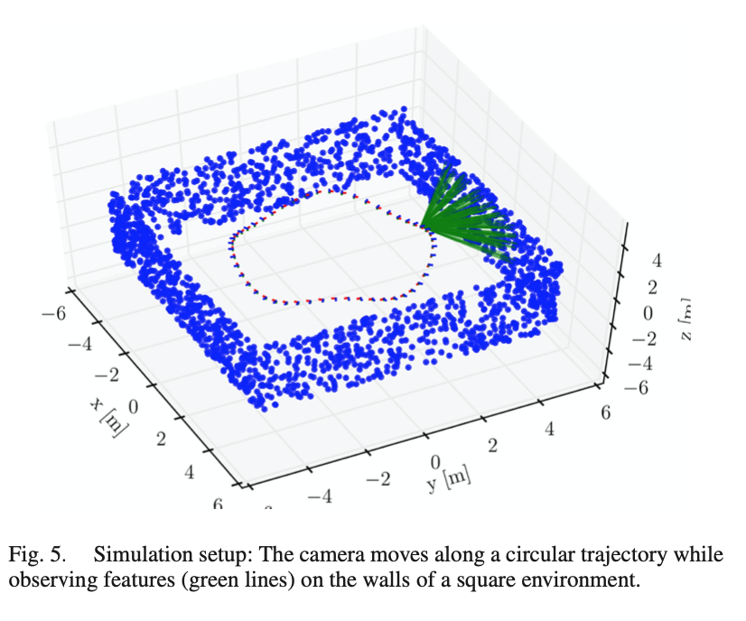
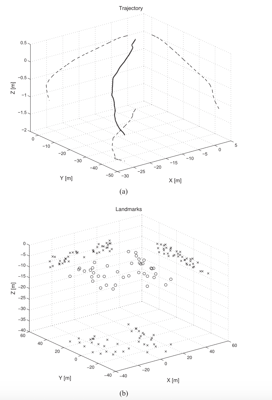
It is common to test and to compare algorithms on synthetic data. Some properties might be more noticeable when we can control the data generating process. In addition, it also helps debugging.
 Forster et al, IEEE Trans. on Robotics, 2017
 Sjanic et al, IEEE Trans. on Aerospace and Electonic Systems, 2017
Step
I layout the steps that we can accomplish the previous graphs.
1. Triangularization
To begin with, we assume that the trajectory is given, and recover the 3D landmark points by the minimizing the cost defined in reprojection_error.h
\(\hat{\lambda} = {arg\,min}_{ {\lambda}}\, \sum_{t=1}^n \| o_t - h_{\pi}(s_t, \lambda) \|^2_{R}.\)
2. Data fusion
After the verification of reprojection_error.h, we can then move to data fusion. In other words, we will minimize the cost function combining the IMU time propagation error and the reprojection error, defined in both reprojection_error.h and imu_error.h.
\((\hat{s}_{1:n}, \hat{\lambda}) = {arg\,min}_{({s}_{1:n}, {\lambda})}\, \sum_{t=0}^{n-1} \| s_{t+1} - f(s_t, u_t) \|^2_{Q} + \sum_{t=1}^n \| o_t - h_{\pi}(s_t, \lambda) \|^2_{R}.\)
3. Covariance matrices
Covariance matrices can be regarded as the weight that we assign for each residuals. With eigen decomposition of covariance matrices, we can scale the residual equations and directly use ceres. This function can be done by NormalPrior by ceres.
4. Local parameterization (optional)
Ceres provides local parameterization to accelerate the optimization process.
Discussion
- the effect of loop closure by giving different trajectories
- the distribution of landmark/feature points