Plate bending, Method of Weighted Residual (MWR), Debugging Trial Function Calculation Method & Free Boundary Condition
Chang LiuRemarks
-
Solving trial function calculation problem. Visually reasonable results achieved with reasonable / faster calculation time. (The problem is when changing symbolic expression to double numerical value, numbers are cut to 17 digits, which is not accurate enough and cause more trouble. The current solution is to change number of digits to 100 and results are more reasonable. The calculation time is longer then using 17 digits, but significantly faster than using null(sym), I would say >95% increase.)
-
Check free boundary conditions, using the new / faster residual calculation method.
-
Stress implemented.
Details
Dec 21, 2020 (Monday)
-
Weird results coming out of trial function calculation. null() function may be misused.
-
Problem: \(null(A_{symbolic})\) is not the same as \(null(A_{double})\). \(null(A_{symbolic}) * A = 0\) and \(null(A_{double}) * A = 0\). \(null(A_{symbolic})\) takes longer time but gives visually correct results. \(null(A_{double})\) is faster but gives visually incorrect results. Technically, we are trying to solve an over-determined linear system, which means there are more equations than variables.
-
Could not find solutions to this problem today, will try tomorrow.
Dec 22, 2020 (Tuesday)
-
Well, following what's left from yesterday, I need to find out why \(null(A_{double})\) doesn't work. (Maybe this is not the problem. Maybe it's somewhere else.) We need to find a solution since \(null(A_{symbolic})\) takes forever to calculate when \(N>11\).
-
The first thing I am trying to do is to check trial function(s) gotten from using \(null(A_{double})\) and \(null(A_{symbolic})\). The trial function(s) should satisfy all boundary conditions at least.
-
\(null(A_{double})\) never gives visually correct answers; \(null(A_{symbolic})\) gives visually correct answers for certain polynomial order; \(null(A_{double}, 'r')\) gives somehow visually correct answers.
-
After some (actually, a lot of) debugging and searching online. I notice the cause for these wrong results may due to the loss of accuracy when converting symbolic numbers to numerical numbers using double() function. double() function only saves 17 digits, which may not be enough. Here are the three method that I tried to calculate trial function coefficients:
%% Method I, this method takes the longest time, but the most actuate
[A, B] = equationsToMatrix(eqn_sum, a);  % note: A and B are symbolic value. Acutally A is symbolic expression (with equations, not results).
coefficient_solution = A \ B + null(A);
coefficient_solution = double(coefficient_solution);
%% Method II, the fastest, but no visually correct results
[A, B] = equationsToMatrix(eqn_sum, a);
A = double(A); % note: this cut the number to ONLY 17 digits, accuracy decreases significantly.
B = double(B);
coefficient_solution = A \ B + null(A, 'r'); % note: low accuracy result.%% Method III,
[A, B] = equationsToMatrix(eqn_sum, a);
digits(100); % note: change numerical/symbolic expression to 100 useful digits.
A = double(A);
A = vpa(A); % note: result in symbolic matrix.
B = double(B);
B = vpa(B);
coefficient_solution = A \ B + null(A); % note: faster calculation than method I, but slower then method II, good accuracy.
coefficient_solution = double(coefficient_solution);-
Checking random 4 edges ploygon, different BC combinations: CSF, CCCC, CSFS,
-
SSSS, SCSC, CCSS, CCFC, SSFC, SCFC.
| Number of edges | Boundary conditions | Polynomial order | Method I time cost (sec) | Method III time cost (sec) | Time increase precentage |
|---|---|---|---|---|---|
| 4 (random) | CSFS | 13 | 1300 | 7.3 | 99.44% |
| 4 (random) | CCSS | 14 | -- | 9 | -- |
Dec 23, 2020 (Wednesday)
- Keep checking more ploygon, different BC combinations: SSF, CFS, SCFC, SCCF
| Number of edges | Boundary conditions | Polynomial order | Method I time cost (sec) | Method III time cost (sec) | Time increase precentage |
|---|---|---|---|---|---|
| 3 (random) | SSF | 8 | 66.78 | N/A | N/A |
| 3 (random) | SSF | 9 | 220.82 | 6.14 | 97.22% |
| 3 (random) | SSF | 10 | 370 | 5.5 | 98.51% |
| 3 (random) | CFS | 9 | 197.36 | 3.97 | 97.98% |
| 3 (random) | CFS | 10 | 371.21 | 5.88 | 98.41% |
| 3 (random) | CFS | 11 | 605.40 | 7.6 | 98.74% |
| 4 (random) | SCFC | 13 | -- | 11.34 | -- |
| 4 (random) | SCFC | 14 | -- | 15.49 | -- |
| 4 (random) | SCFC | 15 | -- | 21.48 | -- |
| 4 (random) | SCCF | 13 | -- | 10.22 | -- |
| 4 (random) | SCCF | 14 | -- | 14.95 | -- |
| 4 (random) | SCCF | 15 | >7200 | 20.97 | -- |
| 4 (random) | SCCF | 16 | -- | 28.47 | -- |
| 4 (random) | SCFF | 13 | -- | 11.3 | -- |
| 4 (random) | SCFF | 14 | -- | 15.92 | -- |
| 4 (random) | SCFF | 15 | -- | 22.75 | -- |
-
After making sure the trial function calculation is correct, I will move on checking free BCs. So far, using the supposed-to-be correct trial function calculation, some examples show visually correct free BC deformation.
-
An interesting but frustrating thing is, using simply-supported BC and free edge BC, results looks normal (positive deformation); using clamped BC and free edge BC, results looks normal (positive deformation); but when using combined simply-supported, clamped and free edge BCs, the results look weird (negative deformation).
Dec 24, 2020 (Thursday)
-
Check free boundary conditions, using the new / faster residual calculation method.
-
Add strain and stress calculation to the code. The strain and stress variables are illustrated in the following figure (I will keep modifying this figure / adding new variables.)
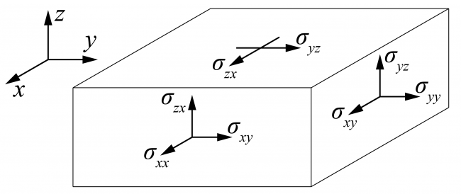
- For stress expressions as functions of deformation \(\omega_{(x, y)}\):
Normal stress:
\(\delta_{xx} = - \frac{E}{1 - \nu^2} z \big( \frac{\partial ^2 \omega}{\partial x ^2} + \nu \frac{\partial ^2 \omega}{\partial y ^2} \big)\)
\(\delta_{yy} = - \frac{E}{1 - \nu^2} z \big( \frac{\partial ^2 \omega}{\partial y ^2} + \nu \frac{\partial ^2 \omega}{\partial x ^2} \big)\)
In-plane shear stress:
\(\delta_{xy} = - \frac{E}{1 - \nu^2} z \frac{\partial ^2 \omega}{\partial x \partial y}\)
Other shear stress
\(\delta_{zx} = - \frac{3 V_x}{2 t} \big( 1 - \big( \frac{z}{t/2} \big)^2 \big)\)
\(\delta_{zy} = - \frac{3 V_y}{2 t} \big( 1 - \big( \frac{z}{t/2} \big)^2 \big)\)
Dec 25, 2020 (Friday)
- Merry Christmas!!
To-Do List
-
Comparison of two plates.
-
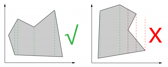
The current implement works for convex polygons, and concave polygons with concaves vertically, but not horizontally. For a simple example:
- ANSYS installation useful links:
https://uasatucla.org/docs/mechanical/tutorials/ansys_setup