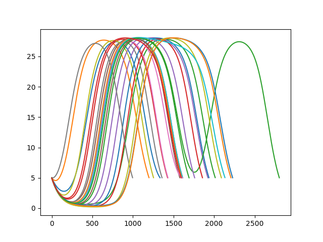
The following is a short overview of the process by which the characteristic velocity of the vehicle is determined from local information. Let \(v(t)\) be the velocity of the vehicle at time \(t\). In the presence of traffic jams, \(v(t)\) will be wave like. A sample of different possible solutions \(v(t)\) are shown below for a characteristic velocity of \(8\)m/s.
Let \(S[v, T]\) be a functional that is continuous in \(T\). If the current traffic jam occurs over an interval of lenght \(T\), then the waveform may be mapped to a vector:
\(x = \left(S_1[v, T], S_2[v, T] , \dots, S_N[v, T] \right)\)
An example is functionals of the form
\(S[v, T] = \int_{0}^{T}\mathcal{L}(v, t)dt\)
where \(\mathcal{L}\) is some nonlinear transformation. This transformation bypasses the problem of system identification in the presence of non-constant lag and allows us to apply standard machine learning tools to identify the characteristic velocity of the system. Currently the transformations being used are
\(S[v, T] = T\)
\(S[v, T] = \frac{1}{T}\int_{0}^{T} v(t)dt\)
\(S[v, T] = \frac{1}{T}\int_{0}^{T}tv(t)dt\)
\(S[v, T] = \frac{v(T) - v(0)}{T}\)
The machine learning solution shows promising results in identifying the characteristic velocity. The next step is to use that as an input to the follower stopper and test whether the resulting autonomous controller can attenuate traffic jams.